I was curious about the bid-ask spread and behavior of contract prices for stock options.
In this notebook I’ll explore a dataset, figure out what data preprations I’ll need, and make basic visualizations to try to support some hypothesis. Along the way I’ll also touch on basics of stock options.
If you want to repeat with your data, note the pandas and numpy version in case you run into errors.
import os
import pandas as pd
from matplotlib import pyplot as plt
import numpy as np
import seaborn as sns
%matplotlib inline
plt.style.use('tableau-colorblind10')
print(f"pandas version {pd.__version__}")
print(f"numpy version {np.__version__}")
pandas version 1.1.3
numpy version 1.19.2
For a few expirations dates in the near future, I exported Apple Inc. (NASDAQ: AAPL) stock option chains into csv files. The prices are a snapshot at the time of this exploration. I first try to open and view one dataframe and decide whether it and other datasets need cleaning.
Note I pass to the read_csv function a comma for semantic indicator of the thousands place.
The next two cells shows information about the AAPL options data as well as a few records. Doing this will let me know what next steps I may need to take in exploration.
df = pd.read_csv(os.path.join(os.getcwd(), 'data', 'AAPL',  'oct-30.csv'), thousands=',')
df.info()
<class 'pandas.core.frame.DataFrame'>
RangeIndex: 78 entries, 0 to 77
Data columns (total 17 columns):
 #   Column        Non-Null Count  Dtype
---  ------        --------------  -----
 0   Trade         77 non-null     object
 1   Quote         77 non-null     object
 2   Open          78 non-null     object
 3   Volume        77 non-null     float64
 4   Net Change    77 non-null     float64
 5   Last          77 non-null     float64
 6   Bid           77 non-null     float64
 7   Ask           77 non-null     float64
 8   Strike        78 non-null     object
 9   Bid.1         77 non-null     float64
 10  Ask.1         77 non-null     float64
 11  Last.1        77 non-null     float64
 12  Net Change.1  77 non-null     float64
 13  Volume.1      77 non-null     float64
 14  Open.1        78 non-null     object
 15  Quote.1       77 non-null     object
 16  Trade.1       77 non-null     object
dtypes: float64(10), object(7)
memory usage: 10.5+ KB
print(df.head(3))
   Trade    Quote      Open  Volume  Net Change   Last    Bid    Ask Strike  \
0    NaN      NaN  Interest     NaN         NaN    NaN    NaN    NaN  Price
1  Trade  Details        98     5.0        1.97  61.02  61.25  61.85     55
2  Trade  Details       263   121.0        1.50  56.35  56.50  56.65     60

   Bid.1  Ask.1  Last.1  Net Change.1  Volume.1    Open.1  Quote.1 Trade.1
0    NaN    NaN     NaN           NaN       NaN  Interest      NaN     NaN
1    0.0   0.01    0.01           0.0       3.0        35  Details   Trade
2    0.0   0.01    0.03           0.0       0.0        31  Details   Trade
Clean up required…
Since I scraped and pasted data from a browser into a csv, there are some browser artifacts I’ll need to take care of that are specific to the way I scrapped the data, namely, row index 0 is probably the result of a table formatting in the browser view, and the Trade and Quote columns are UI elements for the user to click onto the trading page. I’ll need to drop those rows and columns.
Note in the following cells, I create seperate functions because I’m going to demonstrate a data wrangling pipeline with the functions.
def prep_rows(df, row_indices):
    # Just dropping row
    df.drop(index=row_indices)
    return df.drop(index=row_indices)

# drop (row) index 0
df = prep_rows(df, [0])
df.reset_index(inplace=True, drop=True)
print(df.head(3))
   Trade    Quote Open  Volume  Net Change   Last    Bid    Ask Strike  Bid.1  \
0  Trade  Details   98     5.0        1.97  61.02  61.25  61.85     55    0.0
1  Trade  Details  263   121.0        1.50  56.35  56.50  56.65     60    0.0
2  Trade  Details   17     1.0        2.85  51.95  51.50  51.70     65    0.0

   Ask.1  Last.1  Net Change.1  Volume.1 Open.1  Quote.1 Trade.1
0   0.01    0.01           0.0       3.0     35  Details   Trade
1   0.01    0.03           0.0       0.0     31  Details   Trade
2   0.01    0.01           0.0       0.0     36  Details   Trade
The dataframe needs a date column to indicate expiration date of the contract. Also, the table is organized at call options on the left and put options on the right, so I’ll rename all the columns to indicate put or call.
I use some other expressions and structures:
- lambda functions aka anonymous functions to map the column label as a put or call based on whether it has a ‘.1’
- in the lambda function, I do a
value_if_true if condition else value_if_falseaka the ternary operator - to save a little space, the columns holding integers are convert to integers using astype. Commas are removed from strings before conversion. This would have been taken care of when the CSV was read, but the empty row causes some interpretation snags.
- datetime type to write only the date portion of the datetime data type
def prep_columns(df, drop_cols, map_cols, date_label):
    # drop unused columns
    df.drop(columns=drop_cols, inplace=True)

    # add call or put
    df.rename(columns=map_cols, inplace=True)

    # convert everything to numbers
    df.replace(',','', regex=True, inplace=True)

    df = df.astype(float)

    df['call spread'] = df['ask call'] - df['bid call']
    df['put spread'] = df['ask put'] - df['bid put']

    # add date
    df['expire date'] = pd.to_datetime(date_label + "-2020").date()
    return df

drop_cols = ['Trade', 'Quote', 'Quote.1', 'Trade.1']
map_cols = {'Open': 'open interest put',
     'Volume': 'volume call',
     'Net Change': 'net change call',
     'Last': 'last call',
     'Bid': 'bid call',
     'Ask': 'ask call',
     'Strike': 'strike',
     'Volume.1': 'volume put',
     'Net Change.1': 'net change put',
     'Last.1': 'last call',
     'Bid.1': 'bid put',
     'Ask.1': 'ask put',
     'Open.1': 'open interest put',
}
df = prep_columns(df, drop_cols, map_cols, 'oct-30')
df.info()
<class 'pandas.core.frame.DataFrame'>
RangeIndex: 77 entries, 0 to 76
Data columns (total 16 columns):
 #   Column             Non-Null Count  Dtype
---  ------             --------------  -----
 0   open interest put  77 non-null     float64
 1   volume call        77 non-null     float64
 2   net change call    77 non-null     float64
 3   last call          77 non-null     float64
 4   bid call           77 non-null     float64
 5   ask call           77 non-null     float64
 6   strike             77 non-null     float64
 7   bid put            77 non-null     float64
 8   ask put            77 non-null     float64
 9   last call          77 non-null     float64
 10  net change put     77 non-null     float64
 11  volume put         77 non-null     float64
 12  open interest put  77 non-null     float64
 13  call spread        77 non-null     float64
 14  put spread         77 non-null     float64
 15  expire date        77 non-null     object
dtypes: float64(15), object(1)
memory usage: 9.8+ KB
Cleanup pipeline
Now I create a pipeline to so that I can iterate over a list of csv dataset and apply the same functions over each set and append it to the dataframe.
I know the files I’ve created ahead of time so I used those to load the csv’s, transform the data, and append onto the main dataframe. The end result should have 514 rows (again, I counted ahead of time).
dates = ["nov-6", "nov-13", "nov-20", "nov-27", "dec-4", "dec-18"]

for date in dates:
    df2 = pd.read_csv(os.path.join(os.getcwd(), 'data', 'AAPL', date+'.csv'), thousands=',')
    df2 = df2.pipe(prep_rows, [0])\
        .pipe(prep_columns, drop_cols=drop_cols, map_cols=map_cols, date_label=date)
    df = df.append(df2, ignore_index=True)

df.info()
<class 'pandas.core.frame.DataFrame'>
RangeIndex: 514 entries, 0 to 513
Data columns (total 16 columns):
 #   Column             Non-Null Count  Dtype
---  ------             --------------  -----
 0   open interest put  514 non-null    float64
 1   volume call        514 non-null    float64
 2   net change call    514 non-null    float64
 3   last call          514 non-null    float64
 4   bid call           514 non-null    float64
 5   ask call           514 non-null    float64
 6   strike             514 non-null    float64
 7   bid put            514 non-null    float64
 8   ask put            514 non-null    float64
 9   last call          514 non-null    float64
 10  net change put     514 non-null    float64
 11  volume put         514 non-null    float64
 12  open interest put  514 non-null    float64
 13  call spread        514 non-null    float64
 14  put spread         514 non-null    float64
 15  expire date        514 non-null    object
dtypes: float64(15), object(1)
memory usage: 64.4+ KB
print(df.head(3))
   open interest put  volume call  net change call  last call  bid call  \
0               98.0          5.0             1.97      61.02     61.25
1              263.0        121.0             1.50      56.35     56.50
2               17.0          1.0             2.85      51.95     51.50

   ask call  strike  bid put  ask put  last call  net change put  volume put  \
0     61.85    55.0      0.0     0.01       0.01             0.0         3.0
1     56.65    60.0      0.0     0.01       0.03             0.0         0.0
2     51.70    65.0      0.0     0.01       0.01             0.0         0.0

   open interest put  call spread  put spread expire date
0               35.0         0.60        0.01  2020-10-30
1               31.0         0.15        0.01  2020-10-30
2               36.0         0.20        0.01  2020-10-30
🚩
Ok, I’ve done a lot of data manipulation. Let’s graph somethings to see if there are any hint of patterns.
I’ll go ahead and plot the strike prices vs the prices of bid calls and puts. Ignore trying to distinguish between ask and bid right now… I don’t expect that they’ll be too different than what bid call (or put) vs strike price look like.
In general, call options reflect the value of being able to buy a stock at a given strike price of the contract and at the present price of the stock. Conversely, put options reflect the value of being able to sell a stock at a given strike price of the contract and at the present price of the stock.
-
For calls, it’s better to have the choice to buy a stock at a lower price than the actual stock price. You can take advantage of buying at a “discounted” price.
-
For puts, it’s better to have the choice to sell a stock at a higher price than the actual stock price. You can take advantage of selling at a “marked up” price.
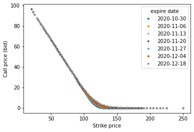
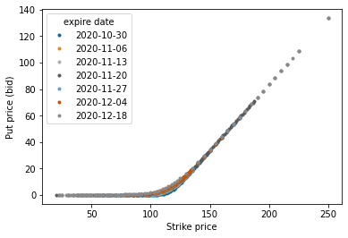
I’ll explain more about those dynamics in the following cells, but first, observe the “hockey stick” shape of the prices. Observe they are mirrors of one another.
df.pivot(index='strike', columns='expire date', values='bid call').plot(marker='.', ls='')
plt.xlabel("Strike price")
plt.ylabel("Call price (bid)")
plt.show()
df.pivot(index='strike', columns='expire date', values='bid put').plot(marker='.', ls='')
plt.xlabel("Strike price")
plt.ylabel("Put price (bid)")
plt.show()
The ins-and-outs of options
Since these numbers are a snapshot of values at a specific point in time i.e. a stock price, we can make some statements that corroborate with reality.
-
Even though I haven’t mentioned the actual stock price, you’d have a fair chance betting that it is somewhere around 120 - 130 dollars if you understand that…
-
For calls, there’s more intrinsic value in being able to buy at prices lower than the actual stock price, or…
-
For puts, there’s more intrinsic value in being able to sell at prices higher than the actual stock price…
-
Passed the actual stock price, there is no intrinsic value in being able to buy the stock at a higher price (for calls). Would you choose to buy a pizza pie at 20 dollars if its advertised price is 15 dollars? The same is true but in the opposite price direction for puts. Would you choose to sell a your boat at 100k if buyers were willing to buy boats at 500k?…
-
Thus, the options' market prices closely track intrinsic values (because no one wants to obvious leave money on the table). The higher the intrinsic value an option, the higher it’s going to be priced at. You can still try to take advantage of the price differential, but the so-call optimization of the market will adjust prices such that you can’t exactly buy a 1 dollar call for a 1001 dollar stock and make 1000 dollars off of it (and vice versa for puts). Passed the actual stock price, the values drop to zero.
🥽 Now onto heavier stuff
Out of all extropolations, the statements above are “low hanging fruit” observations, but I wanted to anchor the data in reality so that I can make more a ambitious explorations.
I have a few hypotheses:
The bid-ask spread of options is correlated with value, and the farther away the strike price, the wider the spread, because there’s less consensus/certainty of the actual stock value reaching the far strike price.
The bid-ask spread of options is correlated with stock volatility. Again, uncertainty causes less consensus in valuation.
So by these hypotheses, a highly volatile stock will have the widest spread at prices far away from the acual stock price.
I know I want to include a graph of the bid-ask spread over strike the domain of strike prices, so I’ll plot strike vs spread for different expiry dates. I’m interested in finding a relationship between strike price and bid ask spread.
Visualization: I use a scatter plot on the spreads for each expiry date. I connect the datapoints so it’s easier to identify which datapoint belongs to which date, but the lines aren’t data interpolation. The disjoint points are a result of limited figure space, and they otherwise should be connected.
df.pivot(index='strike', columns='expire date', values='call spread').plot(marker='.')
plt.title("AAPL call options spread")
plt.xlabel("Strike price")
plt.ylabel("Call spread")
plt.show()
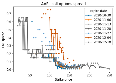
Looks like there’s a trend in the above graph, but it looks a little choppy 🤔. This is because of the values of the prices. Option prices tend to stick to intervals of 0.1.
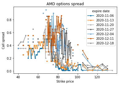
I’ll now bring in more data from AMD (AMD) and Johnson & Johnson (JNJ) to try and glean a pattern across stocks.
df_AAPL = df
dates = ["nov-6", "nov-13", "nov-20", "nov-27", "dec-4", "dec-11", "dec-18"]

df_AMD = pd.DataFrame()
for date in dates:
    df2 = pd.read_csv(os.path.join(os.getcwd(), 'data', 'AMD', date+'.csv'), thousands=',')
    df2 = df2.pipe(prep_rows, [0])\
        .pipe(prep_columns, drop_cols=drop_cols, map_cols=map_cols, date_label=date)
    df_AMD = df_AMD.append(df2, ignore_index=True)
print(df_AMD.info())

df_JNJ = pd.DataFrame()
for date in dates:
    df2 = pd.read_csv(os.path.join(os.getcwd(), 'data', 'JNJ', date+'.csv'), thousands=',')
    df2 = df2.pipe(prep_rows, [0])\
        .pipe(prep_columns, drop_cols=drop_cols, map_cols=map_cols, date_label=date)
    df_JNJ = df_JNJ.append(df2, ignore_index=True)
print(df_AMD.info())
<class 'pandas.core.frame.DataFrame'>
RangeIndex: 402 entries, 0 to 401
Data columns (total 16 columns):
 #   Column             Non-Null Count  Dtype
---  ------             --------------  -----
 0   open interest put  402 non-null    float64
 1   volume call        402 non-null    float64
 2   net change call    402 non-null    float64
 3   last call          402 non-null    float64
 4   bid call           402 non-null    float64
 5   ask call           402 non-null    float64
 6   strike             402 non-null    float64
 7   bid put            402 non-null    float64
 8   ask put            402 non-null    float64
 9   last call          402 non-null    float64
 10  net change put     402 non-null    float64
 11  volume put         402 non-null    float64
 12  open interest put  402 non-null    float64
 13  call spread        402 non-null    float64
 14  put spread         402 non-null    float64
 15  expire date        402 non-null    object
dtypes: float64(15), object(1)
memory usage: 50.4+ KB
None
Create a dataframe for snapshot of the stocks.
df_stock = pd.DataFrame({'symbol': ['AAPL', 'AMD', 'JNJ'],
                         'last price': ['116.60', '76.58','138.50'],
                         'volatility': ['38.15', '50.06', '24.22']})
print(df_stock.head(3))
  symbol last price volatility
0   AAPL     116.60      38.15
1    AMD      76.58      50.06
2    JNJ     138.50      24.22
df_AMD.pivot(index='strike', columns='expire date', values='call spread').plot(marker='.')
plt.title("AMD options spread")
plt.xlabel("Strike price")
plt.ylabel("Call spread")
plt.show()
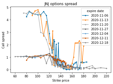
df_JNJ.pivot(index='strike', columns='expire date', values='call spread').plot(marker='.')
plt.title("JNJ options spread")
plt.xlabel("Strike price")
plt.ylabel("Call spread")
plt.show()
Findings 🔎
Observe that while AMD spread has more variance, there’s narrowing tendency as the contracts are specified closer to the current price. The trend is clearer for JNJ stock. This supports my hypothesis that options farther away from strike price have wider spread. I can’t reject that there isn’t a correlation yet, though.
My other hypothesis was about volatility correlating with spread. What it looks like so far is that volatility influences spread such that it varies just as much even as the contract price nears the actual price.
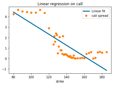
Just for kicks I’ll do a linear regression for JNJ at a specific expiry date and show that the trend line fitted to call data slopes down as we close in on the actual price.
import scipy.stats as sp

sub = df_JNJ[df_JNJ['expire date'] == pd.to_datetime("11-06-2020").date()]
y=np.array(sub['call spread'].values, dtype=float)
x=np.array(sub['strike'].values, dtype=float)
slope, intercept, r_value, p_value, std_err = sp.linregress(x, y)

xf = np.linspace(min(x), max(x), 100)
yf = (slope*xf)+intercept

_, ax = plt.subplots(1, 1)
ax.plot(xf, yf,label='Linear fit', lw=3)
sub.plot(x='strike', y='call spread', ax=ax, marker='o', ls='')
ax.legend()
plt.title("Linear regression on call")
plt.show()
Stay tuned
In the next post continuation, I plan to make more insights and visualizations.
- I have time-series data, so I’ll need to explore its affect on spread.
- The call and put data generally have symmetry in their rules, but are there any assymetrical differences I can uncover in the data?